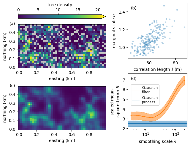
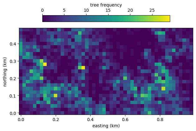
Density of T. panamensis on a 50 ha plot in Panama
Trees on 50 ha plot on Barro Colorado Island have been censused regularly since 1982. The data are publicly available, and we use them here for a demonstration of a Gaussian process using the two-dimensional fast Fourier transform. For a given species, the data comprise the frequency \(y\) of trees in each of 20 by 20 meter quadrants. For this example, we pick T. panamensis because its distribution is relatively heterogeneous over the plot. We load and visualize the data below.
from matplotlib import pyplot as plt
import numpy as np
import os
from pathlib import Path

workspace = Path(os.environ.get("WORKSPACE", os.getcwd()))


# Load the matrix of tree frequencies.
species = "tachve"
frequency = np.loadtxt(f"../../../data/{species}.csv", delimiter=",")
nrows, ncols = frequency.shape
delta = 20 / 1000  # Separation between adjacent plots in km.

# Show the tree frequency in the plot.
fig, ax = plt.subplots()
extent = delta * (np.asarray([0, ncols, 0, nrows]) - 0.5)
im = ax.imshow(frequency, extent=extent, origin="lower")
ax.set_xlabel("easting (km)")
ax.set_ylabel("northing (km)")
fig.colorbar(im, ax=ax, location="top", label="tree frequency", fraction=0.05)
fig.tight_layout()
frequency.shape
(25, 50)
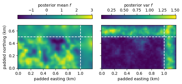
The FFT assumes periodic boundary conditions, but, of course, these do not apply to trees. We thus pad the domain to attenuate correlation between quadrants at opposite sides of the plot. A padding of 10 quadrants corresponds to 200 meters. The model is shown below.
functions {
    #include gptools/util.stan
    #include gptools/fft.stan
}

data {
    // Number of rows and columns of the frequency map and the padded number of rows and columns. We
    // pad to overcome the periodic boundary conditions inherent in fast Fourier transform methods.
    int num_rows, num_cols, num_rows_padded, num_cols_padded;
    // Number of trees in each quadrant. Masked quadrants are indicated by a negative value.
    array [num_rows, num_cols] int frequency;
}

parameters {
    // "Raw" parameter for the non-centered parameterization.
    matrix[num_rows_padded, num_cols_padded] z;
    // Mean log rate for the trees.
    real loc;
    // Kernel parameters and averdispersion parameter for the negative binomial distribution.
    real<lower=0> sigma, kappa;
    real<lower=log(2), upper=log(28)> log_length_scale;
}

transformed parameters {
    real<lower=0> length_scale = exp(log_length_scale);
    // Evaluate the RFFT of the Matern 3/2 kernel on the padded grid.
    matrix[num_rows_padded, num_cols_padded %/% 2 + 1] rfft2_cov =
        gp_periodic_matern_cov_rfft2(1.5, num_rows_padded, num_cols_padded, sigma,
        [length_scale, length_scale]', [num_rows_padded, num_cols_padded]');
    // Transform from white-noise to a Gaussian process realization.
    matrix[num_rows_padded, num_cols_padded] f = gp_inv_rfft2(
        z, rep_matrix(loc, num_rows_padded, num_cols_padded), rfft2_cov);
}

model {
    // Implies that eta ~ gp_rfft(loc, rfft2_cov) is a realization of the Gaussian process.
    to_vector(z) ~ std_normal();
    // Weakish priors on all other parameters.
    loc ~ student_t(2, 0, 1);
    sigma ~ student_t(2, 0, 1);
    kappa ~ student_t(2, 0, 1);
    // Observation model with masking for negative values.
    for (i in 1:num_rows) {
        for (j in 1:num_cols) {
            if (frequency[i, j] >= 0) {
                frequency[i, j] ~ neg_binomial_2(exp(f[i, j]), 1 / kappa);
            }
        }
    }
}
from gptools.stan import compile_model
import os


# Set up the padded shapes.
padding = 10
padded_rows = nrows + padding
padded_cols = ncols + padding

# Sample a random training mask for later evaluation.
seed = 0
np.random.seed(seed)
train_fraction = 0.8
train_mask = np.random.uniform(size=frequency.shape) < train_fraction

# Prepare the data for stan.
data = {
    "num_rows": nrows,
    "num_rows_padded": padded_rows,
    "num_cols": ncols,
    "num_cols_padded": padded_cols,
    # Use -1 for held-out data.
    "frequency": np.where(train_mask, frequency, -1).astype(int),
}

# Compile and fit the model.
model = compile_model(stan_file="trees.stan")
if "CI" in os.environ:
    niter = 10
elif "READTHEDOCS" in os.environ:
    niter = 200
else:
    niter = None
chains = 1 if "READTHEDOCS" in os.environ or "CI" in os.environ else 4
fit = model.sample(data, iter_warmup=niter, iter_sampling=niter, seed=seed, show_progress=False,
                   chains=chains)
print(fit.diagnose())
20:13:41 - cmdstanpy - WARNING - Non-fatal error during sampling:
Exception: neg_binomial_2_lpmf: Location parameter is inf, but must be positive finite! (in '/home/docs/checkouts/readthedocs.org/user_builds/gptools-stan/checkouts/latest/stan/docs/trees/trees.stan', line 46, column 16 to column 74)
	Exception: neg_binomial_2_lpmf: Location parameter is inf, but must be positive finite! (in '/home/docs/checkouts/readthedocs.org/user_builds/gptools-stan/checkouts/latest/stan/docs/trees/trees.stan', line 46, column 16 to column 74)
	Exception: neg_binomial_2_lpmf: Location parameter is inf, but must be positive finite! (in '/home/docs/checkouts/readthedocs.org/user_builds/gptools-stan/checkouts/latest/stan/docs/trees/trees.stan', line 46, column 16 to column 74)
	Exception: neg_binomial_2_lpmf: Location parameter is inf, but must be positive finite! (in '/home/docs/checkouts/readthedocs.org/user_builds/gptools-stan/checkouts/latest/stan/docs/trees/trees.stan', line 46, column 16 to column 74)
Consider re-running with show_console=True if the above output is unclear!
Processing csv files: /tmp/tmp7573sv18/treesgs15jcnc/trees-20230914201246.csv

Checking sampler transitions treedepth.
Treedepth satisfactory for all transitions.

Checking sampler transitions for divergences.
No divergent transitions found.

Checking E-BFMI - sampler transitions HMC potential energy.
E-BFMI satisfactory.

The following parameters had fewer than 0.001 effective draws per transition:
  z[25,49]
Such low values indicate that the effective sample size estimators may be biased high and actual performance may be substantially lower than quoted.

Split R-hat values satisfactory all parameters.

Processing complete.
The model is able to infer the underlying density of trees. As shown in the left panel below, the density follows within the original domain the data but is smoother. Outside the domain, in the padded region delineated by dashed lines, the posterior mean of the Gaussian process is very smooth because there are no data. As shown in the right panel, the posterior standard deviation is small where there is data and large in the padded area without data.
fig, (ax1, ax2) = plt.subplots(1, 2, sharex=True, sharey=True)

padded_extent = delta * (np.asarray([0, padded_cols, 0, padded_rows]) - 0.5)
im1 = ax1.imshow(fit.f.mean(axis=0), extent=padded_extent, origin="lower")
im2 = ax2.imshow(fit.f.var(axis=0), extent=padded_extent, origin="lower")
fig.colorbar(im1, ax=ax1, location="top", label="posterior mean $f$")
fig.colorbar(im2, ax=ax2, location="top", label="posterior var $f$")
ax1.set_ylabel("padded northing (km)")

for ax in [ax1, ax2]:
    ax.set_xlabel("padded easting (km)")
    ax.axhline(nrows * delta, color="w", ls="--")
    ax.axvline(ncols * delta, color="w", ls="--")
fig.tight_layout()
We compare the GP-based inference with a simpler approach that employes a Gaussian filter to smooth the data. The estimate is
from scipy.ndimage import gaussian_filter


def evaluate_scaled_error(actual, prediction, num_bs=1000):
    """
    Evaluate scaled bootstrapped errors between held-out data and model predictions.
    """
    idx = np.random.choice(actual.size, (num_bs, actual.size))
    bs_actual = actual[idx]
    bs_prediction = prediction[idx]
    return (np.square(bs_actual - bs_prediction) / np.maximum(bs_actual, 1)).mean(axis=-1)


def filter_estimate(frequency, train_mask, scale):
    """
    Estimate held-out data using a Gaussian filter.
    """
    smoothed_mask = gaussian_filter(train_mask.astype(float), scale)
    smoothed_masked_frequency = gaussian_filter(np.where(train_mask, frequency, 0), scale)
    return smoothed_masked_frequency / smoothed_mask


# Evaluate predictions and errors using Gaussian filters at different scales.
smoothed_errors = []
sigmas = np.logspace(-0.8, 1)
for sigma in sigmas:
    smoothed_prediction = filter_estimate(frequency, train_mask, sigma)
    smoothed_errors.append(evaluate_scaled_error(frequency[~train_mask],
                                                 smoothed_prediction[~train_mask]))
smoothed_errors = np.asarray(smoothed_errors)


# Also evaluate the errors for the posterior median Gaussian process rates.
rate = np.median(np.exp(fit.stan_variable("f")[:, :nrows, :ncols]), axis=0)
gp_errors = evaluate_scaled_error(frequency[~train_mask], rate[~train_mask])

def plot_errors(smoothed_errors, gp_errors, ax=None):
    """
    Plot bootstrapped errors for Gaussian filter and Gaussian process estimates.
    """
    scale = delta * 1e3  # Show smoothing scale in meters.
    ax = ax or plt.gca()

    # Gaussian filter errors.
    smoothed_loc = smoothed_errors.mean(axis=-1)
    smoothed_scale = smoothed_errors.std(axis=-1)
    line, = ax.plot(scale * sigmas, smoothed_loc, label="Gaussian\nfilter", color="C1")
    ax.fill_between(scale * sigmas, smoothed_loc - smoothed_scale, smoothed_loc + smoothed_scale,
                    alpha=0.5, color=line.get_color())

    # Gaussian process errors.
    gp_loc = gp_errors.mean()
    gp_scale = gp_errors.std()
    line = ax.axhline(gp_loc, label="Gaussian\nprocess")
    ax.axhspan(gp_loc - gp_scale, gp_loc + gp_scale, alpha=0.5, color=line.get_color())

    ax.set_xscale("log")
    ax.set_xlabel(r"smoothing scale $\lambda$")
    ax.set_ylabel("scaled mean-\nsquared error $S$")

plot_errors(smoothed_errors, gp_errors)
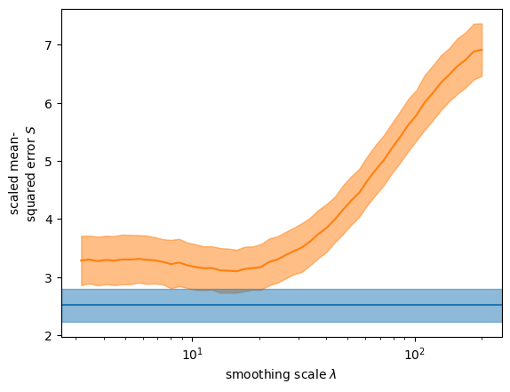
The bootstrapped scaled error for the Gaussian process is lower than the best scaled error for the Gaussian filter—even though the scale of the Gaussian filter was implicitly optimized on the held-out data.
Let’s assemble the parts to produce the figure in the accompanying publication.
import matplotlib as mpl

cmap = mpl.cm.viridis.copy()
cmap.set_under("silver")
kwargs = {
    "origin": "lower",
    "extent": extent,
    "cmap": cmap,
    "norm": mpl.colors.Normalize(0, rate.max()),
}

fig = plt.figure()
fig.set_layout_engine("constrained", w_pad=0.1)
gs = fig.add_gridspec(1, 2, width_ratios=[4, 3])
gs1 = mpl.gridspec.GridSpecFromSubplotSpec(3, 1, gs[0], height_ratios=[0.075, 1, 1])
gs2 = mpl.gridspec.GridSpecFromSubplotSpec(2, 1, gs[1])

cax = fig.add_subplot(gs1[0])
ax1 = fig.add_subplot(gs1[1])
ax1.set_ylabel("northing (km)")
ax1.set_xlabel("easting (km)")
im = ax1.imshow(data["frequency"], **kwargs)

ax2 = fig.add_subplot(gs1[2], sharex=ax1, sharey=ax1)
ax2.set_xlabel("easting (km)")
ax2.set_ylabel("northing (km)")
im = ax2.imshow(rate, **kwargs)

cb = fig.colorbar(im, cax=cax, extend="max", orientation="horizontal")
cb.set_label("tree density")
cax.xaxis.set_ticks_position("top")
cax.xaxis.set_label_position("top")

ax3 = fig.add_subplot(gs2[0])
ax3.scatter(fit.length_scale * delta * 1e3, fit.sigma, marker=".",
            alpha=0.25)
ax3.set_xlabel(r"correlation length $\ell$ (m)")
ax3.set_ylabel(r"marginal scale $\sigma$")

ax4 = fig.add_subplot(gs2[1])
plot_errors(smoothed_errors, gp_errors, ax4)

ax4.legend(fontsize="small", loc=(0.05, 0.425))

fig.draw_without_rendering()

text = ax1.get_yticklabels()[0]
ax1.text(0, 0.5, "(a)", transform=text.get_transform(), ha="right", va="center")
text = ax2.get_yticklabels()[0]
ax2.text(0, 0.5, "(c)", transform=text.get_transform(), ha="right", va="center")
ax3.text(0.05, 0.95, "(b)", va="top", transform=ax3.transAxes)
ax4.text(0.05, 0.95, "(d)", va="top", transform=ax4.transAxes)

fig.savefig(workspace / "trees.pdf", bbox_inches="tight")
fig.savefig(workspace / "trees.png", bbox_inches="tight")