Getting started

This example illustrates the use of gptools by sampling from the prior distribution of a simple Gaussian process model. It uses Fourier Methods to accelerate sampling. Let’s define a squared exponential kernel and the grid \(x\) of \(n\) observations.

from gptools.util.kernels import ExpQuadKernel
from matplotlib import pyplot as plt
import numpy as np


n = 100  # Number of observations.
x = np.arange(n)  # Location of observations.
epsilon = 1e-9  # "Nugget" variance for numerical stability.

# Define a kernel, evaluate the covariance and its Fourier transform.
kernel = ExpQuadKernel(1, n / 10, period=n)
cov = kernel.evaluate(0, x[:, None])
cov[0] += epsilon
cov_rfft = kernel.evaluate_rfft(n) + epsilon

# Show the kernel and its Fourier transform.
fig, (ax1, ax2) = plt.subplots(1, 2)
ax1.plot(x, cov)
ax1.set_xlabel("location $x$")
ax1.set_ylabel("kernel $k(0, x)$")

xi = np.arange(cov_rfft.size)
ax2.plot(xi, cov_rfft)
ax2.set_xlabel(r"frequency $\xi$")
ax2.set_ylabel(r"kernel RFFT $\tilde k(\xi)$")
fig.tight_layout()

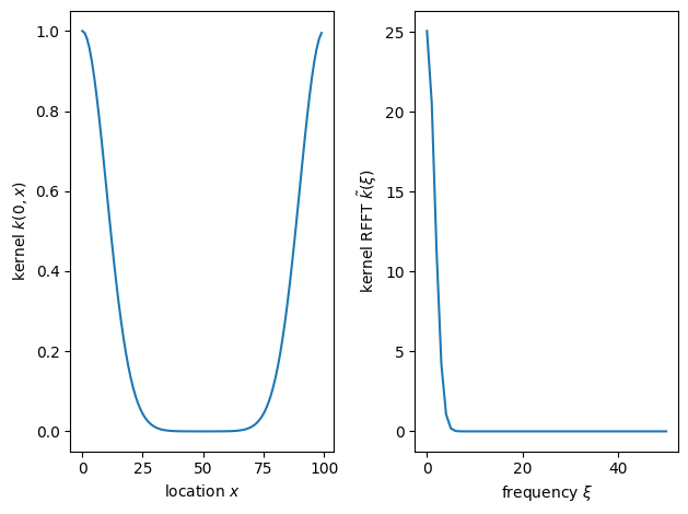
The left panel shows the covariance between a point at \(x=0\) and the rest of the observation grid. We set period=n because the RFFT assumes periodic boundary conditions. While most real-world problems do not have periodic boundary conditions, we can attenuate their effect by padding the domain (see Density of T. panamensis on a 50 ha plot in Panama for details). The right panel shows the Fourier transform of the kernel. Because the squared exponential kernel gives rise to very smooth functions, only the first few Fourier modes have appreciable power. Let’s use Stan to sample from the distribution. The model is shown below.

functions {
    // Include utility functions, such as real fast Fourier transforms.
    #include gptools/util.stan
    // Include functions to evaluate GP likelihoods with Fourier methods.
    #include gptools/fft.stan
}

data {
    // The number of sample points.
    int<lower=1> n;
    // Real fast Fourier transform of the covariance kernel.
    vector[n %/% 2 + 1] cov_rfft;
}

parameters {
    // GP value at the `n` sampling points.
    vector[n] f;
}

model {
    // Sampling statement to indicate that `f` is a GP.
    f ~ gp_rfft(zeros_vector(n), cov_rfft);
}

from gptools.stan import compile_model
import os


# Define a data object for Stan, compile the model, and get the number of samples.
data = {"n": n, "cov_rfft": cov_rfft}
model = compile_model(stan_file="getting_started.stan")

# Sample from the model and visualize samples.
fit = model.sample(data, chains=1, iter_warmup=100, iter_sampling=20)


def plot_samples(fit, alpha):
    fig, ax = plt.subplots()
    ax.plot(x, fit.f.T, color="C0", alpha=alpha)
    ax.set_xlabel("location $x$")
    ax.set_ylabel("GP $f$")
    fig.tight_layout()
    

plot_samples(fit, 0.1)

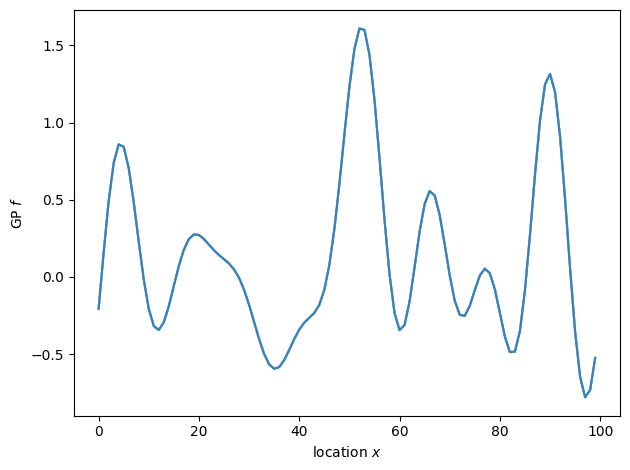
The samples are consistent with a GP prior, but they are far from independent. Under the prior, adjacent elements of \(f\) are heavily correlated. This frustrates Stan’s sampler which draws samples by exploring the target distribution like a ball rolling over a landscape. Narrow valleys lead to slow exploration. We thus need to choose a different parameterization as shown in the model below.

functions {
    // Include utility functions, such as real fast Fourier transforms.
    #include gptools/util.stan
    // Include functions to evaluate GP likelihoods with Fourier methods.
    #include gptools/fft.stan
}

data {
    // The number of sample points.
    int<lower=1> n;
    // Real fast Fourier transform of the covariance kernel.
    vector[n %/% 2 + 1] cov_rfft;
}

parameters {
    // GP value at the `n` sampling points.
    vector[n] z;
}

transformed parameters {
    // Transform from white noise to a GP realization.
    vector[n] f = gp_inv_rfft(z, zeros_vector(n), cov_rfft);
}

model {
    // Implies that `f` is a GP.
    z ~ normal(0, 1);
}

Let’s repeat the sampling process using the reparameterized model.

model = compile_model(stan_file="getting_started_non_centered.stan")
fit = model.sample(data, chains=1, iter_warmup=100, iter_sampling=20)
plot_samples(fit, 0.5)

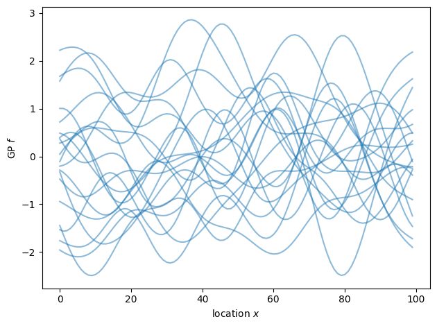
As shown above, we now have virtually independent samples from the target distribution. Picking the right parameterization is important for exploring the target distribution efficiently. You can explore more advanced use cases in further Examples.