Gaussian process Poisson regression

Poisson regression is suitable for estimating the latent rate of count data, such as the number of buses arriving at a stop within an hour or the number of car accidents per day. Here, we estimate the rate using a Gaussian process given synthetic count data. First, we draw the log rate \(\eta\) from a Gaussian process with squared exponential kernel \(k\) observed at discrete positions \(x\), i.e. the covariance of two observations is

\[ \mathrm{cov}\left(\eta(x),\eta(y)\right)=\sigma^2\exp\left(-\frac{d(x, y)^2}{2\ell^2}\right) + \epsilon\delta(x - y), \]

where \(d\left(\cdot,\cdot\right)\) is a distance measure, \(\sigma\) is the marginal scale of the process, and \(\ell\) is its correlation length. The “nugget” variance \(\epsilon\) ensures the covariance matrix is numerically positive semi-definite. Second, we sample counts \(y\) from a Poisson distribution with rate \(\lambda = \exp\eta\). Let’s generate a sample with \(n\) regularly-spaced observations and visualize it.

from gptools.util.kernels import DiagonalKernel, ExpQuadKernel, Kernel
import matplotlib as mpl
from matplotlib import pyplot as plt
import numpy as np


def simulate(x: np.ndarray, kernel: Kernel, mu: float = 0) -> dict:
    """Simulate a Gaussian process Poisson model with mean mu observed at x."""
    # Add an extra dimension to the vector x because the kernel expects an array
    # with shape (num_data_points, num_dimensions).
    X = x[:, None]
    cov = kernel.evaluate(X)
    eta = np.random.multivariate_normal(mu * np.ones_like(x), cov)
    rate = np.exp(eta)
    y = np.random.poisson(rate)
    # Return the results as a dictionary, including input arguments (we need to extract kernel
    # parameters from the `CompositeKernel`).
    return {"x": x, "X": X, "mu": mu, "y": y, "eta": eta, "y": y, "rate": rate, "n": x.size,
            "sigma": kernel.a.sigma, "length_scale": kernel.a.length_scale,
            "epsilon": kernel.b.epsilon}


def plot_sample(sample: dict, ax: mpl.axes.Axes = None) -> mpl.axes.Axes:
    """Visualize a sample of a Gaussian process Poisson model."""
    ax = ax or plt.gca()
    ax.plot(sample["x"], sample["rate"], label=r"rate $\lambda$")
    ax.scatter(sample["x"], sample["y"], marker=".", color="k", label="counts $y$",
               alpha=0.5)
    ax.set_xlabel("Location $x$")
    return ax


np.random.seed(0)
n = 64
x = np.arange(n)
kernel = ExpQuadKernel(sigma=1.2, length_scale=5, period=n) + DiagonalKernel(1e-3, n)
sample = simulate(x, kernel)
plot_sample(sample).legend()

<matplotlib.legend.Legend at 0x7fa3b4358f70>

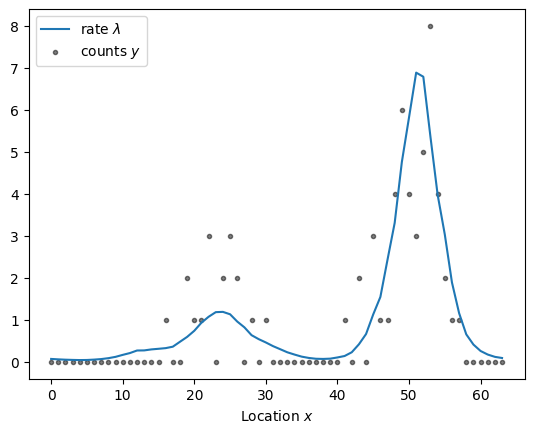
We used a kernel with periodic boundary conditions by passing period=n to the kernel. The Gaussian process is thus defined on a ring with circumference \(n\).

To learn the latent rate using stan, we first define the data block of the program, i.e., the information we provide to the inference algorithm. Here, we assume that the marginal scale \(\sigma\), correlation length \(\ell\), and nugget variance \(\epsilon\) are known.

// Shared data definition for Poisson regression models.

// Kernel parameters.
real<lower=0> sigma, length_scale, epsilon;

// Information about observation locations and counts.
int n;
array [n] int y;
array [n] vector[1] X;

The model is simple: a multivariate normal prior for the log rate \(\eta\) and a Poisson observation model.

// Gaussian process with log link for Poisson observations using the default centered
// parameterization.

data {
    // Shared data definitions.
    #include data.stan
}

parameters {
    // Latent log-rate we seek to infer.
    vector[n] eta;
}

model {
    // Gaussian process prior and observation model. The covariance should technically have periodic
    // boundary conditions to match the generative model in the example.
    matrix[n, n] cov = add_diag(gp_exp_quad_cov(X, X, sigma, length_scale), epsilon);
    eta ~ multi_normal(zeros_vector(n), cov);
    y ~ poisson_log(eta);
}

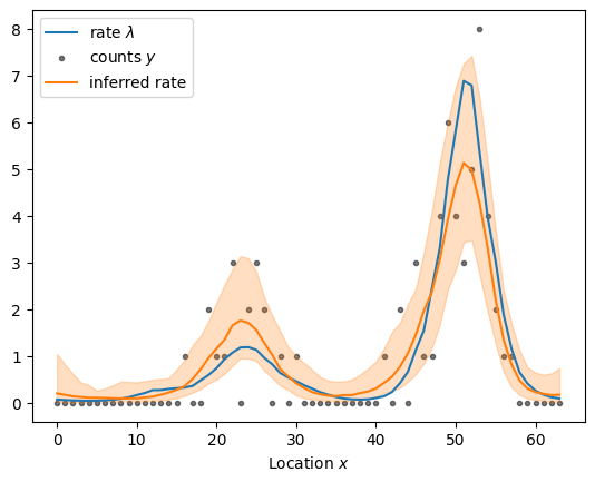
Let’s compile the model, draw posterior samples, and visualize the result.

from cmdstanpy import CmdStanMCMC
from gptools.stan import compile_model
from gptools.util import Timer
from gptools.util.plotting import plot_band
import os


def sample_and_plot(stan_file: str, data: dict, return_fit: bool = False, **kwargs) -> CmdStanMCMC:
    """Draw samples from the posterior and visualize them."""
    # Set default parameters. We use a small number of samples during testing.
    niter = 10 if os.environ.get("CI") else 100
    defaults = {"iter_warmup": niter, "iter_sampling": niter, "chains": 1,
                "refresh": niter // 10 or None}
    defaults.update(kwargs)
    kwargs = defaults

    # Compile the model and draw posterior samples.
    model = compile_model(stan_file=stan_file)
    with Timer(f"sampled using {stan_file}"):
        fit = model.sample(data, **kwargs)

    # Visualize the result.
    ax = plot_sample(sample)
    plot_band(x, np.exp(fit.stan_variable("eta")), label="inferred rate", ax=ax)
    ax.legend()
    if return_fit:
        return fit


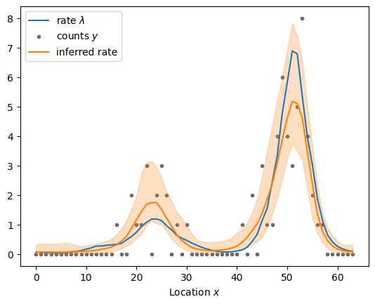
centered_fit = sample_and_plot("poisson_regression_centered.stan", sample, return_fit=True)

sampled using poisson_regression_centered.stan in 11.280 seconds

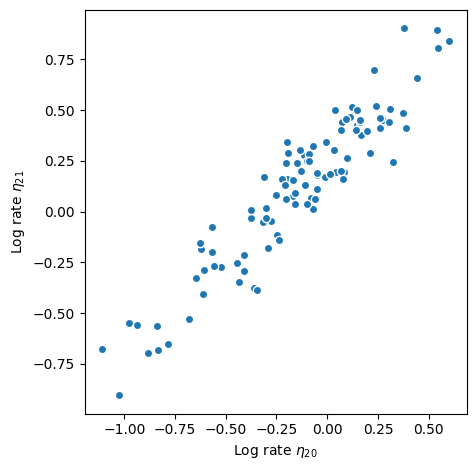
Stan’s Hamiltonian Monte Carlo sampler explores the posterior distribution well and recovers the underlying rate. But it takes its time about it–especially given how small the dataset is. The exploration is slow because adjacenct elements of the log rate are highly correlated under the posterior distribution as shown in the scatter plot below. The mean correlation between adjacent elements is 0.95. The posterior is highly correlated because the Gaussian process prior demands that adjacent points are close: if one moves up, the other must follow to keep the log rate \(\eta\) smooth. If the data are “strong”, i.e., there is more information in the likelihood than in the prior, the data can decorrelate the posterior: each log rate is primarily informed by the corresponding count rather than the prior.

fig, ax = plt.subplots()
etas = centered_fit.stan_variable("eta")
idx = 20
ax.scatter(etas[:, idx - 1], etas[:, idx]).set_edgecolor("w")
ax.set_aspect("equal")
ax.set_xlabel(fr"Log rate $\eta_{{{idx}}}$")
ax.set_ylabel(fr"Log rate $\eta_{{{idx + 1}}}$")
fig.tight_layout()

In this example, the data are relatively weak (recall that the variance of the Poisson distribution is equal to its mean such that, for small counts, the likelihood is not particularly informative). We can alleviate this problem by switching to a non-centered parameterization such that the parameters are uncorrelated under the prior distribution. In particular, we use a parameter \(z\sim\text{Normal}\left(0, 1\right)\) and transform the white noise such that it is a draw from the Gaussian process prior. This approach is a higher-dimensional analogue of sampling a standard normal distribution and multiplying by the standard deviation \(\sigma\) as opposed to sampling from a normal distribution with standard deviation \(\sigma\) directly. The log rate is

\[ \eta = Lz, \]

where \(L\) is the Cholesky decomposition of the covariance matrix \(\Sigma\) of the kernel. The Cholesky decomposition of the covariance matrix is the higher-dimensional analogue of taking the square route of the variance. Because the data are weak, they can only slightly correlate the parameters \(z\). The Stan program is shown below.

// Gaussian process with log link for Poisson observations.

data {
    #include data.stan
}

parameters {
    vector[n] z;
}

transformed parameters {
    vector[n] eta;
    {
        // Evaluate the covariance and apply the Cholesky decomposition to the white noise z. We
        // wrap the evaluation in braces because Stan only writes top-level variables to the output
        // CSV files, and we don't need to store the entire covariance matrix. The covariance should
        // technically have periodic boundary conditions to match the generative model in the
        // example.
        matrix[n, n] cov = add_diag(gp_exp_quad_cov(X, X, sigma, length_scale), epsilon);
        eta = cholesky_decompose(cov) * z;
    }
}

model {
    // White noise prior (implies eta ~ multi_normal(zeros_vector(n), cov)) and observation model.
    z ~ normal(0, 1);
    y ~ poisson_log(eta);
}

non_centered_fit = sample_and_plot("poisson_regression_non_centered.stan", sample, return_fit=True)

sampled using poisson_regression_non_centered.stan in 1.444 seconds

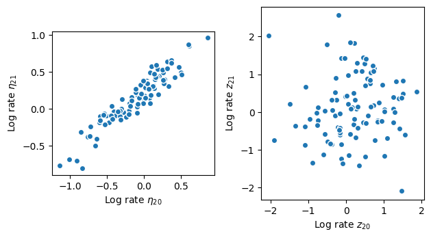
Sampling from the posterior is substantially faster. While the log rates \(\eta\) remain highly correlated (see left panel below), the posterior for the parameters \(z\) the Hamiltonian sampler is exploring are virtually uncorrelated (see right panel below). Takeaway: if the data are strong, use a centered parameterization. If the data are weak, use a non-centered parameterization.

fig, (ax1, ax2) = plt.subplots(1, 2)
etas = non_centered_fit.stan_variable("eta")
zs = non_centered_fit.stan_variable("z")
idx = 20
ax1.scatter(etas[:, idx - 1], etas[:, idx]).set_edgecolor("w")
ax1.set_aspect("equal")
ax1.set_xlabel(fr"Log rate $\eta_{{{idx}}}$")
ax1.set_ylabel(fr"Log rate $\eta_{{{idx + 1}}}$")

ax2.scatter(zs[:, idx - 1], zs[:, idx]).set_edgecolor("w")
ax2.set_aspect("equal")
ax2.set_xlabel(fr"Log rate $z_{{{idx}}}$")
ax2.set_ylabel(fr"Log rate $z_{{{idx + 1}}}$")

fig.tight_layout()

Nearest-neighbor Gaussian processes

Despite the non-centered parameterization being faster, its performance scales poorly with increasing sample size. Evaluating the Cholesky decomposition scales with \(n^3\) such that this approach is only feasible for relatively small datasets. However, intuitively, only local correlations are important for the Gaussian process (at least for the squared exponential kernel we used above). Points separated by a large distance are virtually uncorrelated but these negligible correlations nevertheless slow down our calculations. Fortunately, we can factorize the joint distribution to obtain a product of conditional distributions.

\[ p\left(\eta\mid \Sigma\right)=\prod_{i=1}^n p\left(\eta_{i}\mid\eta_{<i},\Sigma\right), \]

where \(\eta_{<i}\) denotes all parameters \(\left\{\eta_1, \ldots \eta_{i-1}\right\}\) preceeding \(\eta_i\). In a nearest neighbor Gaussian process, we approximate the full conditional by only conditioning on at most the \(k\) preceeding parameters, i.e., we neglect all correlations between parameters that are further apart than the \(k^\text{th}\) nearest neighbor. We thus need to decompose \(n\) square matrices each having \(k + 1\) rows. The computational cost scales as \(nk^3\)–a substantial saving if \(n\) is large compared with \(k\).

More generally, we can construct a Gaussian process on a directed acyclic graph using the factorization into conditionals. Here, we employ this general formulation and represent the nearest neighbor Gaussian process as a graph. The conditioning structure is illustrated below.

from gptools.util.graph import lattice_predecessors, predecessors_to_edge_index

k = 5
predecessors = lattice_predecessors((n,), k)

idx = 20
fig, ax = plt.subplots()
ax.scatter(predecessors[idx, -1] - np.arange(3) - 1, np.zeros(3), color="silver",
           label="ignored nodes")
ax.scatter(idx + np.arange(3) + 1, np.zeros(3), color="silver")
ax.scatter(predecessors[idx], np.zeros(k), label="conditioning nodes")
ax.scatter(idx, 0, label="target node")
ax.legend()
for j in predecessors[idx, :-1]:
    ax.annotate("", xy=(j, 0), xytext=(idx, 0),
                arrowprops={"arrowstyle": "-|>", "connectionstyle": "arc3,rad=.5"})
ax.set_ylim(-.25, .25)
ax.set_axis_off()
fig.tight_layout()

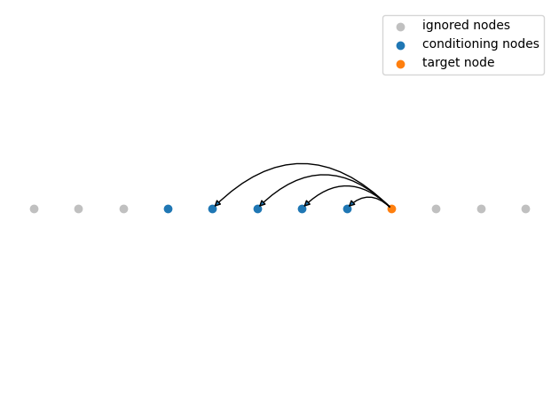
The function lattice_predecessors constructs a nearest neighbor matrix predecessors with shape (n, k + 1) such that the first k elements of the \(i^\text{th}\) row are the predecessors of node \(i\) and the last element is the node itself. The corresponding Stan program is shown below. The distribution gp_graph_exp_quad_cov_lpdf(vector, vector, array [] vector, real, real, array [,] int) encodes the Gaussian process.

// Graph gaussian process with log link for Poisson observations.

functions {
    #include gptools/util.stan
    #include gptools/graph.stan
}

data {
    #include data.stan
    // Information about the graph.
    int num_edges;
    array [2, num_edges] int edge_index;
}

transformed data {
    array [n] int degrees = out_degrees(n, edge_index);
}

parameters {
    vector[n] eta;
}

model {
    // Graph Gaussian process prior and observation model.
    eta ~ gp_graph_exp_quad_cov(zeros_vector(n), X, sigma, length_scale, edge_index, degrees,
                                epsilon);
    y ~ poisson_log(eta);
}

edges = predecessors_to_edge_index(predecessors)
sample.update({"edge_index": edges, "num_edges": edges.shape[1]})
sample_and_plot("poisson_regression_graph_centered.stan", sample)

sampled using poisson_regression_graph_centered.stan in 11.819 seconds

The centered graph Gaussian process is indeed faster than the standard implementation. However, it suffers from the same challenges: the posterior for \(\eta\) is highly correlated. Fortunately, we can also construct a non-centered parameterization.

// Graph gaussian process with log link for Poisson observations.

functions {
    #include gptools/util.stan
    #include gptools/graph.stan
}

data {
    #include data.stan
    // Information about the graph.
    int num_edges;
    array [2, num_edges] int edge_index;
}

transformed data {
    array [n] int degrees = out_degrees(n, edge_index);
}

parameters {
    vector[n] z;
}

transformed parameters {
    // Transform white noise to a sample from the graph Gaussian process.
    vector[n] eta = gp_inv_graph_exp_quad_cov(
        z, zeros_vector(n), X, sigma, length_scale, edge_index, degrees, epsilon);
}

model {
    // White noise prior (implies eta ~ gp_graph_exp_quad_cov(...)) and observation model.
    z ~ normal(0, 1);
    y ~ poisson_log(eta);
}

edges = predecessors_to_edge_index(predecessors)
sample.update({"edge_index": edges, "num_edges": edges.shape[1]})
sample_and_plot("poisson_regression_graph_non_centered.stan", sample)

sampled using poisson_regression_graph_non_centered.stan in 1.489 seconds

The non-centered parameterization of the graph Gaussian process is even faster, and we have reduced the runtime by more than an order of magnitude for this small dataset.

Gaussian process using fast Fourier transforms

If, as in this example, observations are regularly spaced, we can evaluate the likelihood using the fast Fourier transform. Similarly, we can construct a non-centered parameterization by transforming Fourier coefficients with gp_inv_rfft.

// Graph gaussian process with log link for Poisson observations.

functions {
    #include gptools/util.stan
    #include gptools/fft1.stan
}

data {
    #include data.stan
}

parameters {
    vector[n] eta;
}

transformed parameters {
    // Evaluate covariance of the point at zero with everything else.
    vector[n %/% 2 + 1] cov_rfft = gp_periodic_exp_quad_cov_rfft(n, sigma, length_scale, n)
        + epsilon;
}

model {
    // Fourier Gaussian process and observation model.
    eta ~ gp_rfft(zeros_vector(n), cov_rfft);
    y ~ poisson_log(eta);
}

sample_and_plot("poisson_regression_fourier_centered.stan", sample)

sampled using poisson_regression_fourier_centered.stan in 0.881 seconds

sample_and_plot("poisson_regression_fourier_non_centered.stan", sample)

sampled using poisson_regression_fourier_non_centered.stan in 0.182 seconds

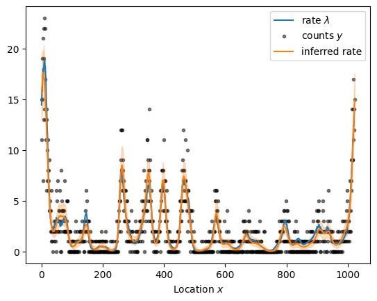
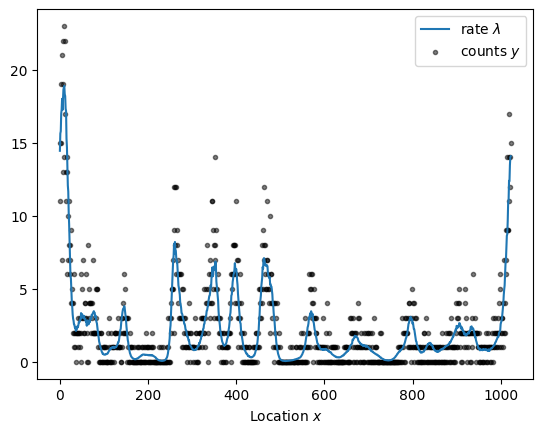
Given the substantial performance improvements, we can readily increase the sample size as illustrated below for a dataset with more than a thousand observations. Sampling from the forward model takes a while because evaluating the periodic squared exponential kernel requires a series approximation.

x = np.arange(1024)
kernel = ExpQuadKernel(sigma=1.2, length_scale=15, period=x.size) + DiagonalKernel(1e-3, x.size)
sample = simulate(x, kernel)
plot_sample(sample).legend()

<matplotlib.legend.Legend at 0x7fa3aaeed870>

sample_and_plot("poisson_regression_fourier_non_centered.stan", sample)

sampled using poisson_regression_fourier_non_centered.stan in 6.715 seconds