Effect and importance of padding

Contrary to most real-world scenarios, the fast Fourier transform and, consequently, Fourier Methods for Gaussian processes assume periodic boundary conditions. This peculiarity can be overcome by padding the domain. This example explores the effect and importance of padding for a simple Gaussian process model. We will draw a sample from a Gaussian process without periodic boundary conditions, \(n\) observations, and squared exponential kernel with correlation length \(\ell\). We will consider how well we can infer it using Fourier methods as a function of the amount of padding \(q\) we use. Padding may, in principle, be introduced anywhere because of the periodic boundary conditions. However, this library has only been tested with padding on the right, as illustrated in the example below.

Before fitting GPs, let’s visualize the kernel on finite domains with different paddings, i.e., we plot the correlation between a point at the origin and another position \(x\).

from gptools.stan import compile_model
from gptools.util.kernels import ExpQuadKernel
from matplotlib import pyplot as plt
import numpy as np


# Declare the number of observations, correlation lengths, and the paddings we want to consider.
num_observations = 128
length_scale = 16
sigma = 1
padding_factors = np.arange(5)

# Then show the kernels with periodic boundary conditions.
fig, ax = plt.subplots()
for factor in padding_factors:
    x = np.arange(num_observations + factor * length_scale)
    kernel = ExpQuadKernel(1, length_scale, period=x.size)
    ax.plot(x, kernel.evaluate(0, x[:, None]), label=fr"padding $q={factor}\times\ell$")
ax.axvline(num_observations, color="k", label="observation domain $n$", ls=":")
ax.legend(loc=(0.175, 0.625))
ax.set_xlabel("location $x$")
ax.set_ylabel("kernel $k(0, x)$")
fig.tight_layout()

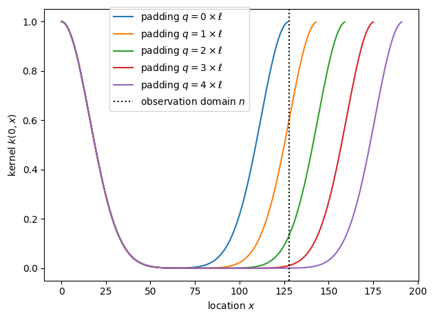
The correlation between opposite sides of the domain is very strong without padding, appreciable for padding with one or two correlation lengths \(\ell\), and becomes small when we pad with three or more correlation lengths.

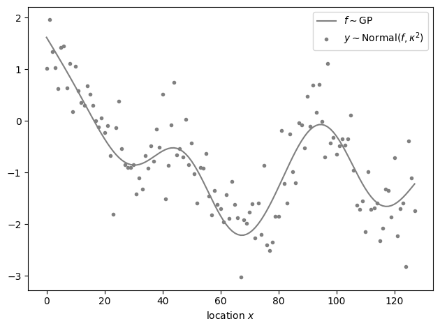
We will draw a Gaussian process sample \(f\) without periodic boundary conditions and use a normal observation model \(y\sim\mathsf{Normal}\left(y,\kappa^2\right)\), where \(\kappa^2\) is the observation variance. We fit the model using two methods: First, the exact but slow model without periodic boundary conditions. Second, a model using Fourier methods with different amounts of padding. We fit all models using the cmdstanpy.CmdStanModel.optimize() method to avoid discrepancies between different fits that arise purely by chance as a result of drawing posterior samples.

# Pick a seed that generates a sample with different values at opposite sides of the domain.
np.random.seed(1)

# Generate a Gaussian process sample.
x = np.arange(num_observations)
kernel = ExpQuadKernel(sigma, length_scale)
cov = kernel.evaluate(x[:, None])
f = np.random.multivariate_normal(np.zeros_like(x), cov)

# Generate noisy observations.
kappa = 0.5
y = np.random.normal(f, kappa)

fig, ax = plt.subplots()
ax.plot(x, f, label=r"$f\sim\mathsf{GP}$", color="gray")
ax.scatter(x, y, marker=".", color="gray", label=r"$y\sim\mathsf{Normal}\left(f,\kappa^2\right)$")
ax.legend()
ax.set_xlabel("location $x$")
fig.tight_layout()

The model for the first method is as follows.

data {
    int num_observations, observe_first;
    int kernel;
    array [num_observations] real x;
    vector[num_observations] y;
    real<lower=0> kappa, length_scale, epsilon, sigma;
}

transformed data {
    cov_matrix[num_observations] cov;
    if (kernel == 0) {
        cov = gp_exp_quad_cov(x, sigma, length_scale);
    } else if (kernel == 1) {
        cov = gp_matern32_cov(x, sigma, length_scale);
    } else {
        reject("kernel=", kernel);
    }
    cov = add_diag(cov, epsilon);
    matrix[num_observations, num_observations] chol = cholesky_decompose(cov);
}

parameters {
    vector[num_observations] z;
}

transformed parameters {
    vector[num_observations] f = chol * z;
}

model {
    z ~ normal(0, 1);
    y[:observe_first] ~ normal(f[:observe_first], kappa);
}

exact_model = compile_model(stan_file="exact.stan")
data = {
    "num_observations": num_observations,
    "x": x,
    "y": y,
    "kappa": kappa,
    "sigma": sigma,
    "length_scale": length_scale,
    "epsilon": 1e-9,
    # We don't use this feature here but consider it in the proper assessment of padding effects
    # to hold out data. See figures/padding-evaluation.md for details.
    "observe_first": num_observations,
    # We only use the squared exponential kernel. See figures/padding-evaluation.md for details.
    "kernel": 0,
}
exact_fit = exact_model.optimize(data)

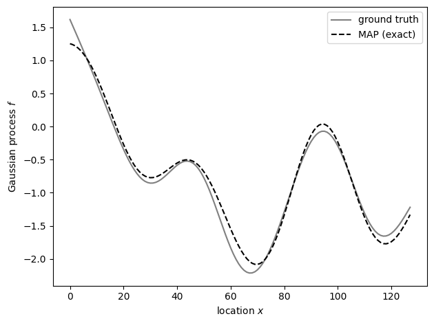
fig, ax = plt.subplots()
ax.plot(x, f, label="ground truth", color="gray")
ax.plot(x, exact_fit.f, label="MAP (exact)", color="k", ls="--")
ax.set_xlabel("location $x$")
ax.set_ylabel("Gaussian process $f$")
ax.legend()
fig.tight_layout()

The model for the second method is as follows.

functions {
    #include gptools/util.stan
    #include gptools/fft1.stan
}

data {
    int num_observations, padding, observe_first;
    int kernel;
    vector[num_observations] y;
    real<lower=0> kappa, length_scale, epsilon, sigma;
}

transformed data {
    int num = num_observations + padding;
    vector[num %/% 2 + 1] cov_rfft;
    if (kernel == 0) {
        cov_rfft = gp_periodic_exp_quad_cov_rfft(num, sigma, length_scale, num);
    } else if (kernel == 1) {
        cov_rfft = gp_periodic_matern_cov_rfft(1.5, num, sigma, length_scale, num);
    }
    cov_rfft += epsilon;
}

parameters {
    vector[num] z;
}

transformed parameters {
    vector[num] f = gp_inv_rfft(z, zeros_vector(num), cov_rfft);
}

model {
    z ~ normal(0, 1);
    y[:observe_first] ~ normal(f[:observe_first], kappa);
}

padded_model = compile_model(stan_file="padded.stan")
data.update({"padding": length_scale * factor})
padded_fits = {}
for factor in padding_factors:
    data.update({"padding": length_scale * factor})
    padded_fits[factor] = padded_model.optimize(data)


fig, ax = plt.subplots()
ax.plot(x, f, label="ground truth", color="gray", zorder=9)
ax.plot(x, exact_fit.f, label="MAP (exact)", color="k", ls="--", zorder=9)
for factor, fit in padded_fits.items():
    f_estimate = fit.f[:num_observations]
    ax.plot(x, f_estimate, label=fr"MAP ($q={factor}\times\ell)$")
    rmse = np.sqrt(np.square(exact_fit.f - f_estimate).mean())
    print(f"RMSE from exact MAP with padding q = {factor} * length_scale: {rmse:.5f}")
ax.set_xlabel("location $x$")
ax.set_ylabel("Gaussian process $f$")
ax.legend()
fig.tight_layout()

RMSE from exact MAP with padding q = 0 * length_scale: 0.28320
RMSE from exact MAP with padding q = 1 * length_scale: 0.04127
RMSE from exact MAP with padding q = 2 * length_scale: 0.00508
RMSE from exact MAP with padding q = 3 * length_scale: 0.00043
RMSE from exact MAP with padding q = 4 * length_scale: 0.00004

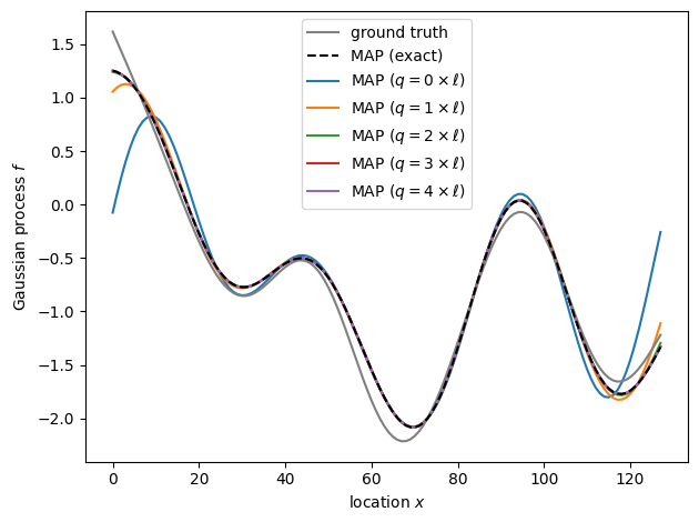
Ignoring the need to pad substantially affects the posterior inference, but we recover the exact MAP estimate well even if we pad with only two correlation lengths. In practice, we often don’t know the correlation length ahead of time, and finding the “right” amount of padding that appropriately balances performance and the need for non-periodic boundary conditions may be an iterative process. For example, we can start with a small amount of padding and increase it until the posterior inference no longer changes.