Passengers on the London Underground network
The London Underground, nicknamed “The Tube”, transports millions of people each day. Which factors might affect passenger numbers at different stations? Here, we use the transport network to build a sparse Gaussian process model and fit it to daily passenger numbers. We first load the prepared data, including features such as the transport zone, number of interchanges, and location, for each station. Detailes on the data preparation can be found here.
We next compile the model and draw posterior samples. The model is shown below.
functions {
    #include gptools/util.stan
    #include gptools/graph.stan
}

data {
    int num_stations, num_edges, num_zones, num_degrees;
    array [num_stations] vector[2] station_locations;
    array [num_stations] int passengers;
    array [2, num_edges] int edge_index;
    matrix[num_stations, num_zones] one_hot_zones;
    matrix[num_stations, num_degrees] one_hot_degrees;
    int include_zone_effect, include_degree_effect;
}

parameters {
    vector[num_stations] z;
    real loc;
    real<lower=0> sigma, kappa;
    real<lower=log(0.32), upper=log(31)> log_length_scale;
    vector[num_zones] zone_effect;
    vector[num_degrees] degree_effect;
}

transformed parameters {
    real length_scale = exp(log_length_scale);
    vector[num_stations] f = gp_inv_graph_exp_quad_cov(
        z, zeros_vector(num_stations), station_locations, sigma, length_scale, edge_index);
    vector[num_stations] log_mean = loc + f
        + include_zone_effect * one_hot_zones * zone_effect
        + include_degree_effect * one_hot_degrees * degree_effect;
}

model {
    z ~ std_normal();
    sigma ~ student_t(2, 0, 1);
    zone_effect ~ student_t(2, 0, 1);
    degree_effect ~ student_t(2, 0, 1);
    kappa ~ student_t(2, 0, 1);
    for (i in 1:num_stations) {
        if (passengers[i] >= 0) {
            log(passengers[i]) ~ normal(log_mean[i], kappa);
        }
    }
}
from gptools.stan import compile_model
import json
import numpy as np
import os


with open("../../../data/tube-stan.json") as fp:
    data = json.load(fp)

# Sample a training mask and update the data for Stan.
seed = 0
train_frac = 0.8
np.random.seed(seed)
train_mask = np.random.uniform(0, 1, data["num_stations"]) < train_frac

# Apply the training mask and include degree and zone effects.
y = np.asarray(data["passengers"])
data.update({
    "include_zone_effect": 1,
    "include_degree_effect": 1,
    # We use -1 for held-out data.
    "passengers": np.where(train_mask, y, -1),
})


if "CI" in os.environ:
    niter = 10
elif "READTHEDOCS" in os.environ:
    niter = 200
else:
    niter = None
model_with_gp = compile_model(stan_file="tube.stan")
chains = 1 if "READTHEDOCS" in os.environ or "CI" in os.environ else 4
fit_with_gp = model_with_gp.sample(data, chains=chains, iter_warmup=niter, iter_sampling=niter,
                                   seed=seed, adapt_delta=0.9, show_progress=False)
print(fit_with_gp.diagnose())
20:14:49 - cmdstanpy - WARNING - Non-fatal error during sampling:
Exception: Exception: Exception: Exception: Exception: gp_exp_quad_cov: magnitude is 0, but must be positive! (in '/home/docs/checkouts/readthedocs.org/user_builds/gptools-stan/checkouts/latest/stan/gptools/stan/gptools/graph.stan', line 54, column 8, included from
	Exception: Exception: Exception: Exception: Exception: gp_exp_quad_cov: magnitude is 0, but must be positive! (in '/home/docs/checkouts/readthedocs.org/user_builds/gptools-stan/checkouts/latest/stan/gptools/stan/gptools/graph.stan', line 54, column 8, included from
	Exception: Exception: Exception: Exception: Exception: gp_exp_quad_cov: magnitude is 0, but must be positive! (in '/home/docs/checkouts/readthedocs.org/user_builds/gptools-stan/checkouts/latest/stan/gptools/stan/gptools/graph.stan', line 54, column 8, included from
Consider re-running with show_console=True if the above output is unclear!
Processing csv files: /tmp/tmpso_zzpg8/tube2tl9ufdi/tube-20230914201420.csv

Checking sampler transitions treedepth.
Treedepth satisfactory for all transitions.

Checking sampler transitions for divergences.
No divergent transitions found.

Checking E-BFMI - sampler transitions HMC potential energy.
E-BFMI satisfactory.

Effective sample size satisfactory.

Split R-hat values satisfactory all parameters.

Processing complete, no problems detected.
We construct a figure that shows the data, effects of zone and degree, and the residual effects captured by the Gaussian process.
from pathlib import Path

fig, axes = plt.subplots(2, 2, gridspec_kw={"width_ratios": [2, 1]}, figsize=(6, 6))
ax1, ax2 = axes[:, 0]
kwargs = {"marker": "o", "s": 10}


X = np.asarray(data["station_locations"])
ax1.scatter(*X[~train_mask].T, facecolor="w", edgecolor="gray", **kwargs)
pts1 = ax1.scatter(*X[train_mask].T, c=y[train_mask], norm=mpl.colors.LogNorm(vmin=np.min(y)),
                   **kwargs)

c = fit_with_gp.stan_variable("f").mean(axis=0)
vmax = np.abs(c).max()
pts2 = ax2.scatter(*X.T, c=c, vmin=-vmax, vmax=vmax,
                   **kwargs, cmap="coolwarm")
ax1.set_aspect("equal")
ax2.set_aspect("equal")

ax2.annotate("Canary Wharf", X[np.argmax(c)], (20, -12), ha="center",
             va="center", fontsize="small",
             arrowprops={"arrowstyle": "->", "connectionstyle": "arc3,rad=-0.5"})
ax2.annotate("Hainault\nLoop", X[np.argmin(c)], (31, 13), ha="right",
             va="center", fontsize="small",
             arrowprops={"arrowstyle": "->", "connectionstyle": "arc3,rad=0.2",
                         "patchA": None, "shrinkA": 10})

ax1.set_axis_off()
ax2.set_axis_off()
location = "top"
fraction = 0.05
cb1 = fig.colorbar(pts1, ax=ax1, label="entries & exits", location=location, fraction=fraction)
cb2 = fig.colorbar(pts2, ax=ax2, label="Gaussian process effect", location=location, fraction=fraction)

for ax in [ax1, ax2]:
    segments = []
    for u, v in np.transpose(data["edge_index"]):
        segments.append([X[u - 1], X[v - 1]])
    collection = mpl.collections.LineCollection(segments, zorder=0, color="silver")
    ax.add_collection(collection)

ax1.set_ylabel("northing (km)")
ax1.set_xlabel("easting (km)")
ax2.set_ylabel("northing (km)")
ax2.set_xlabel("easting (km)")
ax3, ax4 = axes[:, 1]

effect = fit_with_gp.stan_variable("degree_effect")
effect -= effect.mean(axis=1, keepdims=True)
line, *_ = ax3.errorbar(np.arange(effect.shape[1]) + 1, effect.mean(axis=0), effect.std(axis=0),
                        marker="o")
line.set_markeredgecolor("w")
ax3.set_ylabel("degree effect")
ax3.set_xlabel("degree")
ax3.set_xticks([1, 3, data["num_degrees"]])
ax3.set_xticklabels(["1", "3", f"{data['num_degrees']}+"])
ax3.axhline(0, color="k", ls=":")


effect = fit_with_gp.stan_variable("zone_effect")
effect -= effect.mean(axis=1, keepdims=True)
line, *_ = ax4.errorbar(np.arange(effect.shape[1]) + 1, effect.mean(axis=0), effect.std(axis=0),
                        marker="o")
line.set_markeredgecolor("w")
ax4.set_ylabel("zone effect")
ax4.set_xlabel("zone")
ax4.set_xticks([2, 4, data["num_zones"]])
ax4.set_xticklabels(["2", "4", f"{data['num_zones']}+"])
ax4.axhline(0, color="k", ls=":")

ax1.text(0.025, 0.05, "(a)", transform=ax1.transAxes)
ax2.text(0.025, 0.05, "(c)", transform=ax2.transAxes)
ax3.text(0.05, 0.95, "(b)", transform=ax3.transAxes, va="top")
ax4.text(0.95, 0.95, "(d)", transform=ax4.transAxes, va="top", ha="right")


fig.tight_layout()

workspace = Path(os.environ.get("WORKSPACE", os.getcwd()))
fig.savefig(workspace / "tube.pdf", bbox_inches="tight")
fig.savefig(workspace / "tube.png", bbox_inches="tight")
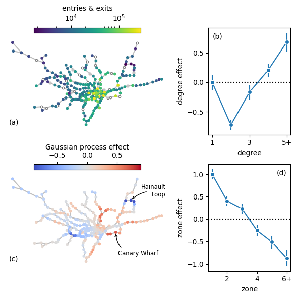
On the one hand, the three northern stations of the Hainault Loop (Roding Valley, Chigwell, and Grange Hill) are underused because they are serviced by only three trains an hour whereas nearby stations (such as Hainault, Woodford, and Buckhurst Hill) are serviced by twelve trains an hour. On the other hand, Canary Wharf at the heart of the financial district has much higher use than would be expected for a station that only serves a single line in zone 2.