Logistic regression

This notebook illustrates the use of the gptools-stan package by fitting a univariate latent Gaussian process (GP) to synthetic binary outcomes. It comprises three steps:

1. generating synthetic data from the model.

2. defining the model in Stan using the Fourier methods provided by the package.

3. fitting the model to the synthetic data and analyzing the results.

Generating synthetic data

We consider a latent Gaussian process \(z(x)\) on a regular grid \(x\) which encodes the log odds of binary outcomes \(y\). More formally, the model is defined as

\[\begin{split}\begin{aligned} z&\sim\mathsf{MultivariateNormal}\left(0, K\right)\\ y&\sim\mathsf{Bernoulli}\left(\mathrm{expit} (z)\right), \end{aligned}\end{split}\]

where \(\mathrm{expit}(z) = 1/\left(1 + \exp(-z)\right)\) denotes the logistic sigmoid and \(K\) is the covariance matrix between elements of the Gaussian process evaluated on the grid. Specifically, we use a squared exponential kernel \(k\) such that

\[\begin{split}\begin{aligned} K_{ij}&=k\left(x_i,x_j\right) + \epsilon \delta_{ij}\\ &=\sigma^2\exp\left(-\frac{\left\vert x_i - x_j\right\vert}{2\ell^2}\right), \end{aligned}\end{split}\]

where \(\sigma\) is the marginal scale of the Gaussian process and \(\ell\) is the correlation length of the kernel. We add a so-called “nuggest variance” \(\epsilon={10}^{-6}\) to the diagonal of the covariance matrix to ensure it is numerically positive definite.

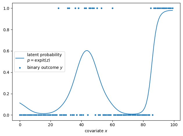
For the synthetic data, we consider \(n=100\) regularly spaced observations, a relatively large correlation length \(\ell=10\) to illustrate the smoothing effect of GPs, and marginal scale \(\sigma=2\).

from matplotlib import pyplot as plt
import numpy as np
from scipy import special


# Define hyperparameters.
n = 100
sigma = 2
length_scale = 10
epsilon = 1e-6
seed = 0

# Seed random number generator for reproducibility, create grid, and generate synthetic data.
np.random.seed(seed)
x = np.arange(n)
cov = sigma ** 2 * np.exp(- (x[:, None] - x[None, :]) ** 2 / (2 * length_scale ** 2)) \
    + epsilon * np.eye(n)
z = np.random.multivariate_normal(np.zeros_like(x), cov)
proba = special.expit(z)
y = np.random.binomial(1, proba)

The figure below shows the latent probability for a positive outcome as a curve and individual observation as a scatter plot. We seek to infer the former given the latter.

def plot_synthetic_data(x, y, proba, ax=None):
    ax = ax or plt.gca()
    ax.plot(x, proba, label="latent probability\n$p=\\mathrm{expit}\\left(z\\right)$")
    ax.scatter(x, y, label="binary outcome $y$", marker=".")
    ax.set_xlabel("covariate $x$")

fig, ax = plt.subplots()
plot_synthetic_data(x, y, proba)
ax.legend()
fig.tight_layout()

Defining the model in Stan

We employ gptools-stan to approximate the GP using Fourier methods (see Fourier Methods for theoretical background). Fourier methods induce periodic boundary conditions, and we need to introduce padding \(p\) to attenuate their effect (see Effect and importance of padding for details). Here, we pad the domain with the number of observations, i.e., the padded domain has \(m=2n\) grid points, which is sufficient to overcome boundary effects.

Each binary outcome only contains a limited amount of information (think of trying to estimate whether a coin is fair by only flipping it once). The latent GP \(z\) is thus only weakly constrained by the data such that adjacent point are highly correlated under the posterior distribution. We use a non-centered parameterization of the GP which is more efficient for weakly constrained GPs (see Parameterizations for details and the “Reparameterization” section of the Stan user guide for a general discussion).

To complete the model, we need to specify priors for the marginal scale \(\sigma\) and correlation length \(\ell\). We use a half-normal distribution for the former. Specifying a prior for the latter can be challenging: The correlation length is not identifiable when it is smaller than the separation between adjacent points or larger than the domain (see the case study “Robust Gaussian Process Modeling” for details). Here, we use a log-uniform prior on the interval \((2, n / 2)\) to restrict the correlation length.

The complete model is shown below.

functions {
    #include gptools/util.stan
    #include gptools/fft1.stan
}

data {
    int n, p;
    array [n] int y;
    real<lower=0> epsilon;
}

transformed data {
    int m = n + p;
}

parameters {
    real<lower=0> sigma;
    real<lower=log(2), upper=log(n / 2.0)> log_length_scale;
    vector[m] raw;
}

transformed parameters {
    real length_scale = exp(log_length_scale);
    // Evaluate the covariance kernel in the Fourier domain. We add the nugget
    // variance because the Fourier transform of a delta function is a constant.
    vector[m %/% 2 + 1] cov_rfft = gp_periodic_exp_quad_cov_rfft(
        m, sigma, length_scale, m) + epsilon;
    // Transform the "raw" parameters to the latent log odds ratio.
    vector[m] z = gp_inv_rfft(raw, zeros_vector(m), cov_rfft);
}

model {
    // White noise implies that z ~ GaussianProcess(...).
    raw ~ normal(0, 1);
    y ~ bernoulli_logit(z[:n]);
    sigma ~ normal(0, 3);
    // Implicit log uniform prior on the length scale.
}

generated quantities {
    vector[n] proba = inv_logit(z[:n]);
}

Fitting the model and analyzing results

We fit the model in two steps. First, we compile the model using the compile_model() wrapper for cmdstanpy. The function ensures include paths are configured appropriately such that gptools-stan can be included using Stan’s #include syntax. If you intend to use a different interface, the library path needs to be added to the include_paths of the interface (see the cmdstanpy documentation for details). The library path can be obtained by running python -m gptools.stan from the command line. Second we call the sample method of the compiled model to obtain posterior samples.

from gptools.stan import compile_model


model = compile_model(stan_file="logistic_regression.stan")
data = {
    "n": n,
    "p": n,
    "y": y,
    "epsilon": epsilon,
}
fit = model.sample(data, seed=seed, show_progress=False)
print(fit.diagnose())

Processing csv files: /tmp/tmpi7eva6c7/logistic_regressionvahks4mm/logistic_regression-20230914200704_1.csv, /tmp/tmpi7eva6c7/logistic_regressionvahks4mm/logistic_regression-20230914200704_2.csv, /tmp/tmpi7eva6c7/logistic_regressionvahks4mm/logistic_regression-20230914200704_3.csv, /tmp/tmpi7eva6c7/logistic_regressionvahks4mm/logistic_regression-20230914200704_4.csv

Checking sampler transitions treedepth.
Treedepth satisfactory for all transitions.

Checking sampler transitions for divergences.
No divergent transitions found.

Checking E-BFMI - sampler transitions HMC potential energy.
E-BFMI satisfactory.

Effective sample size satisfactory.

Split R-hat values satisfactory all parameters.

Processing complete, no problems detected.

Finally, we can visualize the inferred probability curve (shown in orange in the left panel with a band representing the posterior interquartile range) and compare it with the synthetic GP we generated (in blue).

fig, (ax1, ax2) = plt.subplots(1, 2, width_ratios=[3, 2])

plot_synthetic_data(x, y, proba, ax1)
lower, center, upper = np.quantile(fit.proba, [0.25, 0.5, 0.75], axis=0)
line, = ax1.plot(x, center, label="inferred latent\nprobability")
ax1.fill_between(x, lower, upper, color=line.get_color(), alpha=0.2)
ax1.legend(fontsize="small", loc=(0.05, .7))

ax2.scatter(fit.length_scale, fit.sigma, marker=".", alpha=0.2)
ax2.scatter(length_scale, sigma, marker="X", color="k", edgecolor="w")
ax2.set_xlabel(r"length scale $\ell$")
ax2.set_ylabel(r"marginal scale $\sigma$")

fig.tight_layout()

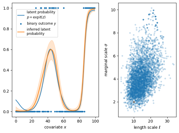
The panel on the right shows posterior samples of the correlation length \(\ell\) and marginal scale \(\sigma\) of the kernel. The parameter values used to generate the data are shown as a black cross and are consistent with posterior samples. However, the kernel parameters remain weakly identified because the binary observations are not very informative.